Page 1

AI Strategy

AI Paradoxes: Why Human Expertise is the Ultimate Moat

A technical deep dive into the failure modes of pure automation.

Posted by Julian Quernheim on February 17, 2026

Over the last few months, I have published several LinkedIn posts and short articles regarding the counter-intuitive nature of machine learning. I have now written this comprehensive article to collect and summarize my findings.

When working with Data Science in the real world, ML models often fail despite high validation accuracy. These failures usually stem from fundamental paradoxes that mathematical optimization alone cannot solve. These paradoxes are not new, but how we deal with these issues becomes more and more vital as Data science is being commoditized. As we move toward autonomous AI agents, understanding these friction points is the only way to build reliable systems.

The Architect's View: AI operates on high-dimensional embeddings and statistical proximity. It excels at mapping known relationships but lacks the causal grounding required for high-stakes edge cases.

1. Moravec’s Paradox: The Reasoning vs. Perception Gap

Hans Moravec observed that high-level reasoning—logic, algebra, and strategy—requires very little computation. In contrast, low-level sensorimotor skills like walking or object recognition require massive computational resources. This is why an LLM can write a complex Spark optimization script in seconds but a robot struggles to navigate a cluttered room.

For us, this means "Human-in-the-loop" is most valuable at the edges of perception and physical interaction. Logic is easy to automate; common sense is computationally expensive and difficult to encode in a loss function.

2. Simpson’s Paradox: The Causality Trap

Machine Learning models are correlation engines. They struggle with the "Causal Ladder." Simpson’s Paradox occurs when a trend in subgroups reverses when the data is aggregated. Mathematically, for variables $A, B$ and a hidden confounder $C$:

$$P(A|B, C) > P(A|B^c, C) \text{ and } P(A|B, C^c) > P(A|B^c, C^c) \text{, but } P(A|B) < P(A|B^c)$$

To interpret this equation, look at the contrast between the conditional probabilities. The left side shows that treatment $B$ outperforms $B^c$ within every specific segment of the population (both $C$ and $C^c$). However, the final term reveals a total reversal: in the aggregate, $B$ appears inferior. In a Data Science context, this usually signals that the confounder $C$ is a weighting variable. If your model recommends a marketing spend based on aggregate ROI, it might miss that the spend is actually underperforming in every individual demographic once the data is segmented. Without causal grounding, the algorithm "punishes" a variable for the inherent difficulty of the segment it was tested in.

3. The Ellsberg Paradox: Ambiguity and the Black Box

This paradox proves that humans prefer known risks over unknown probabilities (ambiguity). We mitigate this using Explainable AI (XAI). Using SHAP (Shapley Values), we can quantify the contribution $\phi_i$ of each feature by evaluating it across all possible feature subsets $S$:

$$\phi_i(f,x) = \sum_{S \subseteq N \setminus \{i\}} \frac{|S|! (M - |S| - 1)!}{M!} [f(S \cup \{i\}) - f(S)]$$

The logic of this formula rests on the marginal contribution, represented by the difference $[f(S \cup \{i\}) - f(S)]$. This measures how the model's prediction shifts when feature $i$ is introduced to a specific subset of other features. Because the order in which features are introduced changes their impact, the combinatorial weight—the fraction involving factorials—averages these contributions fairly across all possible permutations. For a practitioner, this turns an ambiguous "Black Box" into a transparent system by identifying exactly which feature "moved the needle" for a specific prediction, effectively resolving the user's aversion to unknown model logic.

4. The Peltzman Effect: The Hidden Risk of Guardrails

Safety measures often change human behavior. In AI, this is known as risk compensation. When we implement strict output filters or safety layers, users stop verifying the model’s work. They assume the system is "safe." This is particularly dangerous in software development. Developers merging AI-generated PRs often skip unit tests because the code syntax is perfect, even if the logic contains subtle race conditions that a manual coder would have caught.

5. Ramsey Theory: Finding Order in Noise

Ramsey Theory states that in any sufficiently large system, complete disorder is impossible. Structures and patterns must appear by mathematical necessity. This is the "Big Data" curse: with enough dimensions, an AI will find a statistically significant correlation between any two variables by pure chance.

$$R(k, l) \le \binom{k+l-2}{k-1}$$

The Ramsey Number $R(k, l)$ represents the minimum dataset size required to guarantee a specific internal structure. The binomial coefficient on the right side of the inequality illustrates the exponential growth of potential connections as the dataset $N$ grows. In high-dimensional spaces, this means a model is mathematically "forced" to find patterns, regardless of whether they represent physical reality. As Data Scientists, we must distinguish these "Ramsey artifacts" from true signals using cross-validation and bootstrapping, ensuring our findings aren't just a byproduct of the sheer volume of data.


Summary: AI is built for scale and pattern recognition. Humans are built for causal reasoning and ethical oversight. The most successful systems in the next decade won't be fully autonomous; they will be those where the Data Scientist acts as a "Causal Auditor," separating mathematical noise from reality.
How AI Agents Talk: LangGraph + MCP

From multi-agent workflows to real-world voice bots for project acquisition

Posted by Julian Quernheim on August 20, 2025

In recent years, AI has shifted from being about single, monolithic assistants to teams of agents that can coordinate their work. Two technologies that make this collaboration possible are LangGraph, which structures agent workflows, and the Model Context Protocol (MCP), which standardizes how agents exchange information. Together, they allow us to build systems where multiple AI agents can communicate and act in harmony.

I have worked with these technologies in practice. For one project, I built a voice bot for project acquisition that schedules appointments with potential clients. This bot combined LangGraph for orchestration, OpenAI Realtime for low-latency conversations, and LangFuse for session tracking and logging. The result was a system where a user could call in, interact naturally, and walk away with a confirmed appointment—powered by several agents working behind the scenes.

The remainder of this article answers the following three questions:

  • How do LangGraph and MCP enable multi-agent communication?
  • How can they be applied in real-world projects like a voice bot?
  • What does the future look like for agent-based AI systems?

1. How do LangGraph and MCP enable communication?

LangGraph models AI systems as a graph of nodes. Each node can be an agent, tool, or service, and edges define the flow of messages. This makes it possible to design workflows where one agent retrieves information, another interprets it, and a third presents it back to the user. Feedback loops, fallbacks, and parallel tasks all become manageable within this structure.

MCP complements LangGraph by defining the protocol agents use to talk to each other. Instead of custom adapters, every agent sends and receives standardized message types (prompts, tool calls, results). This ensures interoperability, allowing you to swap in new components without breaking the system.

2. A real-world use case: the appointment scheduling voice bot

In my project, the LangGraph workflow defined a chain of responsibilities:

  • A Voice I/O node converted between speech and text in real time.
  • A Dialogue Manager node interpreted intent and handled branching flows (e.g., rescheduling, confirming availability).
  • A Scheduling node integrated with calendars to find open slots.
  • A Logging node (via LangFuse) tracked the entire session for analysis and debugging.

All of these nodes communicated using MCP messages. LangGraph orchestrated the flow—who talks to whom and in what order—while OpenAI Realtime ensured the user experienced a natural, human-like conversation. The system successfully booked appointments with potential clients, freeing up human time for higher-value interactions.

3. The bigger picture

Nowadays, AI agents have become a commodity. Many companies now offer user-friendly interfaces where a custom voice bot can be designed in just a few hours. However, serious deployments still require expertise: fine-tuning, compliance, integrations, and scaling all take longer. As large language models (LLMs) approach their limits, the focus shifts to orchestration, personalization, and governance—the very strengths of frameworks like LangGraph and MCP.

We are quickly reaching a threshold of what raw LLMs can do alone. The future lies in how we connect them: combining models, tools, and data sources into agent-based ecosystems that solve real business problems.


Recurrent Neural Networks applied to predict stock market data

How do recurrent neural networks work and how can we apply them to time‑series data to make predictions about the future?

Posted by Julian Quernheim on January 06, 2019

I have recently studied how neural networks work on sequential data. In particular, I applied a neural network to stock market data to predict the behaviour of a stock over time. This article describes how recurrent neural networks are built, trained, and used for forecasting. For the impatient readers, you can find the source code in my git repository.

A recurrent neural network (RNN) is an artificial neural network (ANN) that can be applied to sequential data, which makes it a perfect candidate for time‑series analysis and an alternative to more conventional methods such as (S)ARIMA.

The remainder of this article answers the following three questions:

  • How does an RNN work?
  • How is an RNN trained?
  • How can we apply an RNN to forecast stock prices?

1. How does an RNN work?

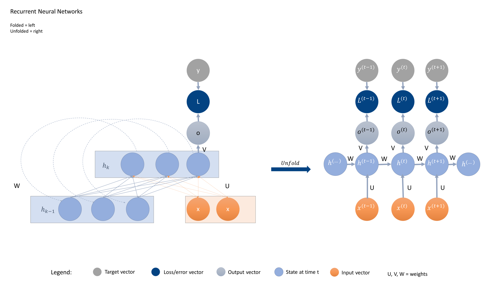
Like any other ANN, RNNs consist of input, hidden, and output layers. Each layer consists of many nodes, which are connected to all nodes in the next layer or, in the case of RNNs, also to itself (recurrency).

Since RNNs allow the previous output to be used as input while having additional hidden states, they are often applied in, for example, speech recognition or forecasting problems. They are typically presented in a folded or unfolded way as shown below.

RNN diagram

The most important building block of any artificial neural network is the perceptron. The perceptron is a simple algorithm for learning a binary classifier that maps an input vector $x$ to a binary output value $f(x)$. With regard to neural networks, the perceptron is said to ‘activate’ or ‘deactivate’ a neuron. In mathematical terms this implies:

$$ f(x) = f\big(b + \sum_{i=1}^m x_i\,\theta_i\big) $$

With regard to recurrent neural networks, we add some more complexity to the model. But despite the additional time dimension, the fundamental building blocks of an RNN stay identical to an ANN. Hence, for an RNN the activation of the hidden neuron $h^{(t)}$ for each timestamp $t$ is defined as: $$h^{(t)} = f_{(h)}(Ux^{(t)} + Wh^{(t-1)} + b_{(h)} )$$ where $U$ and $W$ are the weights, $b$ is the bias term and $f$ is the activation function (e.g., sigmoid, tanh or ReLU).

2. How is an RNN trained?

The objective of an RNN is to minimise the sum of the global loss/error vector $$ \mathbf L = \sum_{t=1}^T L^{(t)} $$ by adjusting the weight matrices $W$, $U$ and $V$ accordingly. These weights are attached to the edges of the neural network and determined during training using an algorithm called Backpropagation Through Time (BPTT) (Werbos, 1990). Like any other optimisation problem, we need to calculate the gradient of the global loss w.r.t. the weights. Hence, the gradient of the loss is defined by $$ \frac{\partial L}{\partial \mathbf W} = \sum_{t=1}^T \frac{\partial L^{(t)}}{\partial \mathbf W}. $$

Next, we apply the chain rule and write the gradient as

$$ \frac{\partial L}{\partial \mathbf W} = \sum_{t=1}^T \sum_{k=1}^t \frac{\partial L^{(t)}}{\partial \mathbf o^{(t)}} \frac{\partial \mathbf o^{(t)}}{\partial \mathbf h^{(t)}} \frac{\partial \mathbf h^{(t)}}{\partial \mathbf h^{(k)}} \frac{\partial \mathbf h^{(k)}}{\partial \mathbf W} . $$

Here $\mathbf o^{(t)}$ is the output vector at time $t$, $\mathbf h^{(t)}$ is the hidden vector at time $t$, and $\mathbf h^{(k)}$ is the hidden vector of node $k$ at time $t$. Note that $\frac{\partial \mathbf h^{(t)}}{\partial \mathbf h^{(k)}}$ depends on time, which implies that the more historic data are considered, the more gradients need to be computed. For long time series, the BPTT algorithm might run into the vanishing or exploding gradient problem because many matrix multiplications can cause the gradient to shrink to zero or explode to infinity.

3. How can we apply an RNN to forecast stock prices?

Applying Recurrent Neural Networks (RNNs) to financial forecasting transforms a standard regression problem into a sequence-to-sequence modeling task. The core advantage of an RNN—specifically its Gated Recurrent Unit (GRU) or Long Short-Term Memory (LSTM) variants—is its ability to maintain a "hidden state" that acts as a memory, capturing the temporal dependencies and momentum inherent in stock market data. Unlike traditional models that treat each day as an independent data point, the RNN processes a sliding window of historical prices to predict the next value in the series.

The implementation process begins with Data Preprocessing. Financial data is notoriously noisy and non-stationary. To make it suitable for a neural network, the data must be normalized (typically using Min-Max scaling) to a range between 0 and 1. This prevents larger values (like total volume) from dominating the gradients during the training process. The dataset is then structured into overlapping sequences. For instance, if we want to predict the price on Day 11 based on the previous 10 days, our input $x$ is a vector of prices from $[t-10, ..., t-1]$, and our target $y$ is the price at $t$.

The Architecture Design usually involves stacking multiple LSTM or GRU layers to extract hierarchical features from the time-series. The first layer might capture short-term fluctuations, while deeper layers identify long-term trends or cyclical patterns. A Dropout layer is frequently integrated between these recurrent layers to prevent overfitting—a common pitfall in finance where models "memorize" historical noise rather than learning generalizable patterns.

During the Training Phase, we utilize the Backpropagation Through Time (BPTT) algorithm. The model compares its prediction against the actual closing price using a Loss Function like Mean Squared Error (MSE). Optimization algorithms, such as Adam or RMSprop, then adjust the weight matrices $U, W,$ and $V$ to minimize this error.

Finally, in the Inference and Evaluation stage, the model is tested on "out-of-sample" data. It is crucial to use a walk-forward validation approach rather than a random split, as maintaining the chronological order is essential for a realistic backtest. While the RNN can capture complex non-linearities that ARIMA models miss, practitioners often combine these forecasts with sentiment analysis or macroeconomic indicators to build a truly robust trading agent.


  • Werbos, P. (1990): Backpropagation Through Time: What It Does and How to Do It. https://doi.org/10.1109/5.58337 Retrieved from http://axon.cs.byu.edu/~martinez/classes/678/Papers/Werbos_BPTT.pdf

Hackathon 2017 Munich: Fake news classifier

How to identify fake news and build a simple web application with Python?

Posted by Julian Quernheim on July 16, 2017

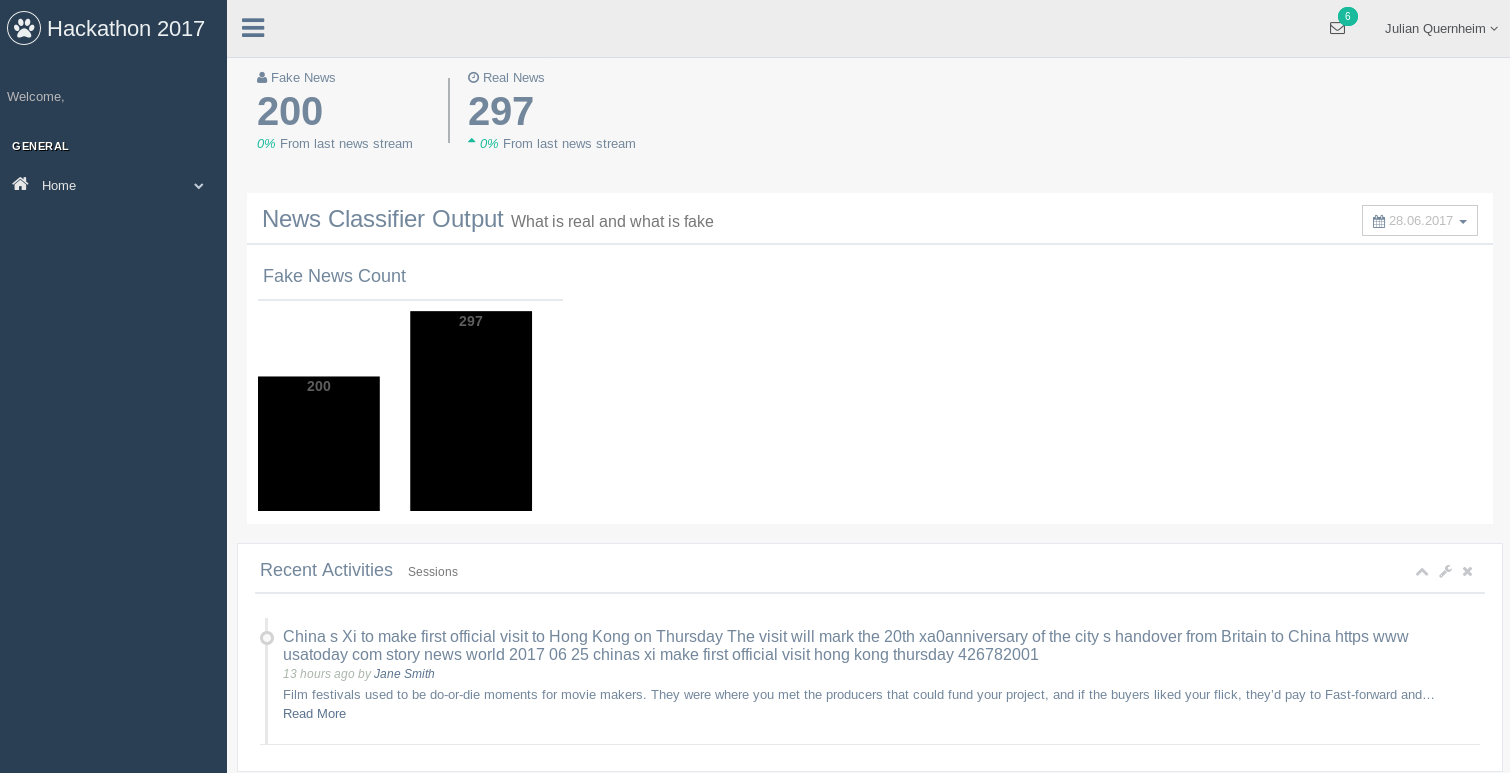
Last month I participated in the Global Hackathon 2017 in Munich, which gave me a whole weekend to dedicate to a data science problem. This year, I decided to build a fake news classifier app with Python.

We worked together to solve the problem of determining if a news article is fake or real. After a little brainstorming, we quickly came up with an idea using a combination of natural language pre‑processing, supervised machine‑learning algorithms and a good‑looking front‑end web application.

The full stack consists of the natural language processing library (nltk), the famous data‑science library (scikit‑learn), a webserver library (Flask) and some basic HTML, CSS and JavaScript.

The remainder of this article answers the following three questions:

  • How to create features out of text?
  • How to build a text classifier model and how to predict the class of a new news article?
  • How to build a website hosted with a Python web application?

For those who cannot wait to see some code and to play around with the final fake news classifier web application, visit my git repository and clone it. The README explains how to run the application in an isolated Docker container.

Fake news app screenshot

1. How to create features out of text?

Text files, such as news articles, should be treated no differently than well‑structured datasets with rows and columns for applying machine‑learning algorithms. The path to preprocess text files into meaningful numerical features is, however, a little bit tricky.

2. Clean your data and convert text data into a weighted term–document frequency matrix (TF‑IDF)

The first step is to load all news articles into matrix form, called a document–term matrix, where each row represents the document id and each column the individual words present in the entire article corpus. Each cell therefore shows the word count within each article.

Since some words, such as stopwords, appear more often than others, the relative importance of each word must be calculated next. Therefore, we multiply the document–term matrix by the inverse of the word frequency count vector. Thus, words with high frequency in the entire corpus are penalised and less frequent words gain more importance in determining the meaning of the article.

The term frequency–inverse document frequency is calculated as $$\mathrm{TFIDF}(t,d,D) = \mathrm{TF}(t) \times \mathrm{IDF}(t)$$ $$\mathrm{TFIDF}(t,d,D) = \frac{f_{t,d}}{\sum f_{t,d}} \times \log \frac{|D|}{\sum_{D: t \in D} 1}$$

TF$(t)$ = (Number of times term $t$ appears in a document) / (Total number of terms in the document).
IDF$(t)$ = $\log_e$(Total number of documents / Number of documents with term $t$ in it).

Show me the script

3. Train a classifier model

Training the statistical model is actually the most straightforward task. Within the module, I define the model type in the __init__.py file, which is loaded as soon as the module loads from within main.py. In this case I chose a random forest classifier because it performed best during testing. You can change the model by modifying the variable model_type to execute the corresponding model.

Show me the script

4. Stream new news and predict their class (fake vs. real)

The final step is to use the statistical model to classify news articles. The script stream_news.py downloads new articles from https://newsapi.org and analyses their likelihood of being fake or real. It loads the stored model model.pkl from disk and applies it to the new articles, each in turn within the function getDailyNews(). Note that we have to clean and transform each news article into a format that can be used as input for our model. This is where the TF‑IDF transformation is applied again.

Show me the script

Lastly, the prediction is stored as a CSV file on disk for later retrieval.

Concluding remarks

Building a complete smart data product that is able to classify news headlines into fake and real was an interesting task for a weekend. The approach focused more on the reusability of the result than on the ultimate accuracy of the statistical model. Having a baseline model which uses random forest classification to measure similarity between the two groups is a good start.


Face Recognition With Python

How does face detection work?

Posted by Julian Quernheim on April 1, 2017

Face recognition is easy for humans, but until today little is known about how we actually perform this task. Our brain trains individual nerve cells to respond to specific features of a scene, such as lines, angles or edges. Our visual cortex then combines these features into meaningful information. Here we focus on a data‑driven approach to face recognition using Python and scikit‑learn.

There are several types of image recognition methods. One intuitive approach is based on geometric features of an image: during training you extract marker points (e.g. positions of eyes or ears) and build a feature vector. Predictions are then based on Euclidean distances.

There is a very good tutorial on keypoint detection at Kaggle: link to Kaggle.

Another face recognition method is based on Eigenfaces. In a nutshell, each image (its pixels) is transformed into eigenvectors via principal component analysis (PCA). The combination of all eigenvectors represents the eigenface.

For more information, please visit Scholarpedia: link to Scholarpedia.

Automatic face recognition is about extracting meaningful features from an image, storing them in a useful representation and performing classification on them. Four tasks are involved:

  1. Find all faces in a picture. Convert the image to greyscale and compute local gradients (e.g. HOG). Compare against a trained HOG face pattern.
  2. Project and pose faces. Handle different angles or illumination via landmark alignment (eyes, ears, nose) and rotation/scale normalisation.
  3. Encode faces with a deep network. Train a model to extract the most meaningful characteristics. PCA/eigenfaces can also be used.
  4. Identify the person. Use a classifier (e.g. SVM or logistic regression) on the encodings to predict identities.

I focused on building the classifier to predict the name of the person, reusing existing models for detection and alignment.

The script below is adapted from the scikit‑learn example (link to scikit).

Show me the script
Enterprise Architecture

Real-Time Analytics: Architecting for Scalability & Cost

Posted by Julian Quernheim

For modern organizations, data is no longer a static asset—it is a continuous stream. However, the architectural "tax" of processing this stream can quickly spiral out of control. To optimize for both performance and cost, we must evaluate the structural design principles of our data pipelines through the lens of Total Cost of Ownership (TCO).

1. The Lambda Architecture: Stability at a Price

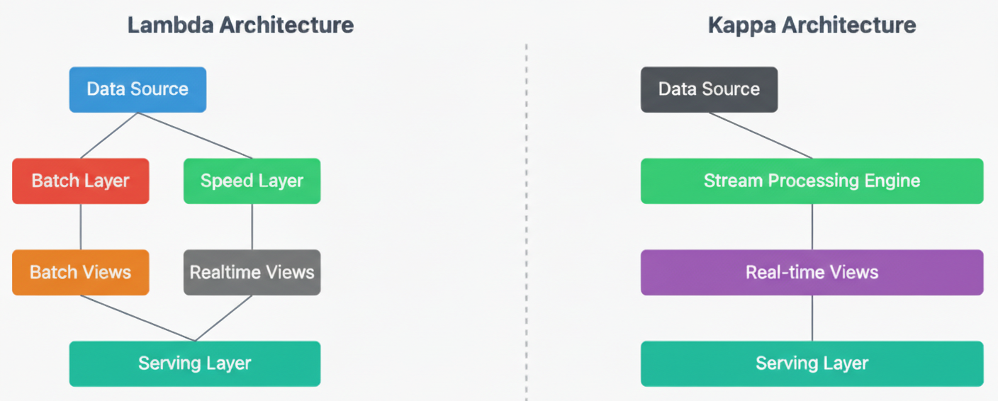
The Lambda Architecture is the traditional "belt-and-suspenders" approach. It attempts to provide both low-latency results and high-accuracy historical data by maintaining two separate processing paths: the Speed Layer and the Batch Layer.

Organizational Impact: While Lambda offers high fault tolerance, it significantly increases Technical Debt. Teams must maintain two different codebases—often one in Spark for batch and one in Flink for streaming—leading to "Logic Drift" where the two layers produce slightly different results for the same query. This creates a hidden cost in data reconciliation and audit hours.

Hence, maintenance costs in Lambda are inherently high. TCO can be double, since logic must be written, tested, and deployed twice.

2. The Kappa Architecture: Streamlining for Agility

The Kappa Architecture proposes a radical simplification: Everything is a stream. By utilizing a high-throughput unified log like Apache Kafka, we eliminate the batch layer entirely. Historical data is simply "replayed" through the streaming engine whenever logic changes are deployed.

lambda_vs_kappa diagram

Design Principles for Cost Saving:

  • Single Codebase: High-level abstractions e.g. Python classes or libraries allow developers to write logic once. This reduces development and maintenance overhead by approximately 40%.
  • Unified Data Governance: By consolidating on a single platform, organizations reduce the "Integrity Tax"—the resources spent reconciling disparate data sources.

3. The Presentation Layer: Scaling the "Last Mile"

The complexity of streaming doesn't end at the database; it extends to the user's browser. High-frequency data (100+ events/sec) can easily crash a standard web dashboard due to Main Thread Jitter and DOM bottlenecks.

To maintain cost-efficiency, we shift the heavy lifting to the Client-Side using Plotly’s optimized rendering. By utilizing the extendTraces method, we achieve Constant Time Complexity $O(1)$ for UI updates. This prevents the browser from slowing down as more data points are added over time.

The Memory Constraint: Even in efficient UI layers, memory $M$ must be capped to prevent leaks. We implement a sliding window where: $$M_{client} \approx \text{Event Rate} (\lambda) \times \text{Window Size} (W)$$

Summary of Trade-offs

Metric Lambda Kappa
Implementation Dual Codebase (High Debt) Unified (High Agility)
Operational Cost High (Redundant Compute) Low (Consolidated)
Use Case Ad-hoc complex analytics Real-time products/viz
// Optimization: O(1) update to prevent DOM bottleneck
function streamToDashboard(newData) {
    Plotly.extendTraces('graph-div', {
        y: [[newData.value]],
        x: [[newData.time]]
    }, [0], 1000); // Capped at 1000 points to ensure O(1) performance
}

Data Exploration With Shiny

Explore your data interactively

Posted by Julian Quernheim on March 1, 2017

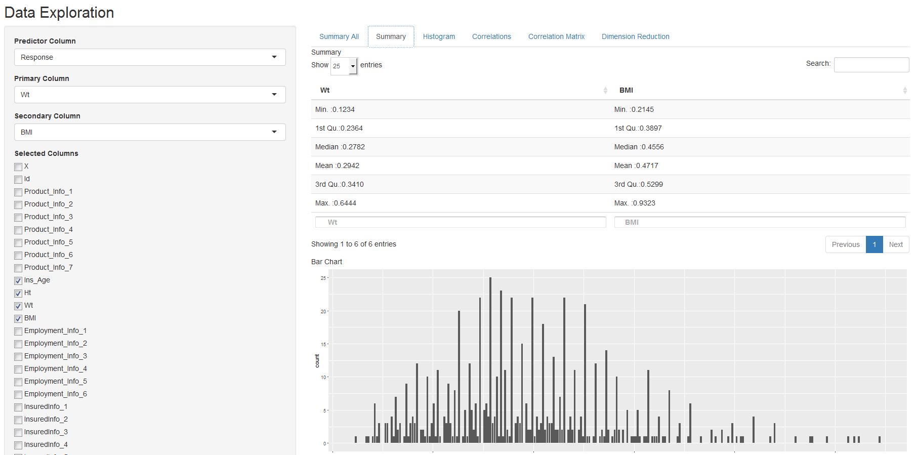
Selecting the right information from a dataset is difficult. Wouldn't it be great to have a data exploration and feature selection tool at your disposal to simplify the work? Shiny is a rapid application development package for R.

I developed a Shiny app to simplify visual data exploration. Since Shiny provides the UI structure, you still use R packages such as ggplot2/ggally for visualisation or boruta for feature selection. You can also integrate custom JavaScript libraries like D3.

Shiny app

Shiny separates the graphical user interface structure (ui.R), the server logic (server.R) and the startup script. For convenience, all three parts can be in one script.

Show me the script


Page 1 of 3